PGFs in NumPy
PGFs in NumPy
Recall our algorithm to find the distribution of $S_n$, the sum of $n$ i.i.d. copies of a random variable $X_1$ that has values in a finite set of non-negative integers.
- Start with the pgf of $X_1$.
- Raise it to the power $n$. That's the pgf of $S_n$.
- Read the distribution of $S_n$ off the pgf.
In this section we will use NumPy to carry out this algorithm.
Suppose the distribution of $X_1$ is given by $p_0 = 0.1$, $p_1 = 0.5$, $p_2 = 0.4$. Let probs_X1 be an array containing the probabilities of the values 0, 1, and 2.
probs_X1 = make_array(0.1, 0.5, 0.4)
dist_X1 = Table().values(np.arange(3)).probability(probs_X1)
Plot(dist_X1)
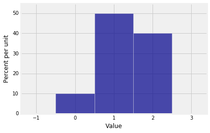
The pgf of $X_1$ is $$ 0.1 + 0.5s + 0.4s^2 $$
NumPy expresses this polynomial in the standard mathematical way, leading with the term of the highest degree:
The method np.flipud reverses the array of probabilities to be consistent with this order of coefficients. The ud in the name is for "up down". NumPy is thinking of the array as a column.
coeffs_X1 = np.flipud(probs_X1)
coeffs_X1
The method np.poly1d takes the array of coefficients as its argument and constructs the polynomial. The 1d in the name stands for "one dimensional".
pgf_X1 = np.poly1d(coeffs_X1)
print(pgf_X1)
The call to print displays the polynomial in retro typewriter style, using $x$ where we have been using $s$. Keep in mind that the final term is the coefficient of $x^0$.
Now suppose $S_3$ is the sum of three i.i.d. copies of $X_1$. The pgf of $S_3$ is the cube of the pgf of $X_1$ and can be calculated just as you would hope.
pgf_S3 = pgf_X1**3
print(pgf_S3)
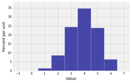
The possible values of $S_3$ are 0 through 6 because $S_3$ is the sum of three copies of a variable that takes values 0 through 2. The coefficients are the probabilities in the distribution of $S_3$.
You can extract an array of the coefficients by using a polynomial attribute called c for "coefficients".
coeffs_S3 = pgf_S3.c
coeffs_S3
These are the probabilities of the values 6 down to 0. In probability theory it is more natural to think of the probabilities of values in the sequence 0 through 6, so use np.flipud again:
probs_S3 = np.flipud(coeffs_S3)
probs_S3
You now have the inputs you need for drawing the probability histogram of $S_3$.
dist_S3 = Table().values(np.arange(7)).probability(probs_S3)
Plot(dist_S3)
A Function to Calculate the Distribution of $S_n$
We will combine the steps above to create a function dist_sum that takes as its arguments the number of terms $n$ and the probabilities in the distribution of $X_1$, and returns the distribution of the sum of $n$ i.i.d. copies of $X_1$.
def dist_sum(n, probs_0_through_N):
    """Return the distribution of S_n,
    the sum of n i.i.d. copies
    of a random variable with distribution probs_0_through_N
    on the integers 0, 1, 2, ..., N"""

    # Find the possible values of S_n
    N = len(probs_0_through_N) - 1
    values_Sn = np.arange(n*N + 1)

    # Find the probailities of those values
    coeffs_X1 = np.flipud(probs_0_through_N)
    pgf_X1 = np.poly1d(coeffs_X1)
    pgf_Sn = pgf_X1**n
    coeffs_Sn = pgf_Sn.c
    probs_Sn = np.flipud(coeffs_Sn)

    t = Table().with_columns(
        'Value', values_Sn,
        'Probability', probs_Sn
    )
    return t
The Sum of the Numbers on $n$ Rolls of a Die
In Chapter 3 we found the exact distribution of the sum of five rolls of a die by listing all $6^5$ possible outcomes and computing the sum for each of them. That method gets intractable with larger numbers of rolls. Let's see if our new method can find the distribution of the sum of 10 rolls of a die.
We have to start with the distribution of a single roll, for which it is important to remember to include 0 as the probability of 0 spots. Otherwise the pgf will be wrong because NumPy won't know that it is not supposed to include a term of degree 0.
die = np.append(0, (1/6)*np.ones(6))
die
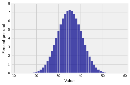
Plot(dist_sum(1, die))
Plot(dist_sum(10, die))
Making Waves
The distribution of the sum of 10 rolls of a die looks beautifully normal. Do all sums have roughly normal distributions?
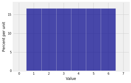
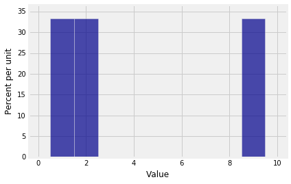
To explore this question, let $X_1$ have the distribution given by $p_1 = p_2 = p_9 = 1/3$.
probs_X1 = make_array(0, 1/3, 1/3, 0, 0, 0, 0, 0, 0, 1/3)
Here is the distribution of $X_1$.
Plot(dist_sum(1, probs_X1))
The probability histogram of $S_{10}$ shows that sums don't always have smooth distributions.
Plot(dist_sum(10, probs_X1))
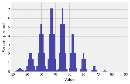
The distribution of $S_{30}$ looks like a stegosaurus having a bad hair day.
Plot(dist_sum(30, probs_X1))
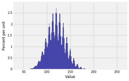
And the distribution of $S_{100}$ is ...
Plot(dist_sum(100, probs_X1))
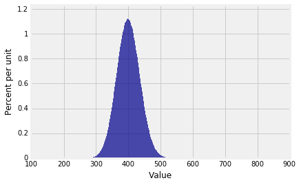
... beautifully normal.
It's begining to look as though there's a theorem here. In the rest of the chapter we will study that theorem, which about the approximate distribution of the sum of a large i.i.d. sample.
Keep in mind that our pgf method gives the exact distribution of the sum of an i.i.d. sample from a distribution on finitely many non-negative integers, provided NumPy can handle the calculations. In the example above, the pgf of $S_{100}$ is a polynomial of degree 900. NumPy handled it just fine.