Odds Ratios
Odds Ratios
Binomial $(n, p)$ probabilities involve powers and factorials, both of which are difficult to compute when $n$ is large. This section is about a simplification of the computation of the entire distribution. The result also helps us understand the shape of binomial histograms.
Consecutive Odds Ratios
Fix $n$ and $p$, and let $P(k)$ be the binomial $(n, p)$ probability of $k$. That is, let $P(k)$ be the chance of getting $k$ successes in $n$ independent trials with probability $p$ of success on each trial.
For $k \ge 1$, define the $k$th consecutive odds ratio $$ R(k) = \frac{P(k)}{P(k-1)} $$
To see how this helps us calculate each $P(k)$ without having to calculate factorials and powers each time, notice that
\begin{align*} P(0) &= (1-p)^n \\ \\ P(1) &= P(0) \cdot \frac{P(1)}{P(0)} = P(0)R(1) \\ P(2) &= P(0)R(1)R(2) \end{align*}and so on.
How is this more illuminating than plugging into the binomial formula? To see this, fix $k \ge 1$ and calculate the ratio $R(k)$.
\begin{align*} R(k) &= \frac{\binom{n}{k}p^k(1-p)^{n-k}} {\binom{n}{k-1}p^{k-1}(1-p)^{n-k+1}} \\ \\ &= \frac{n-k+1}{k} \cdot \frac{p}{1-p} ~~~ \text{(after cancellation)} \\ \\ &= \big{(} \frac{n+1}{k} - 1 \big{)} \cdot \frac{p}{1-p} \end{align*}First, notice that the formulas for $R(k)$ are simple. For example, if $n \ge 3$, it is easy to calculate $P(3)$ as
$$ P(3) = (1-p)^n \cdot \frac{n - 1 + 1}{1} \cdot \frac{p}{1-p} \cdot \frac{n - 2 + 1}{2} \cdot \frac{p}{1-p} \cdot \frac{n - 3 + 1}{3} \cdot \frac{p}{1-p} \cdot $$No factorials involved.
Shapes of Binomial Histograms
Now observe that comparing $R(k)$ to 1 tells us whether the histogram is going up, staying level, or going down at $k$.
\begin{align*} R(k) > 1 &\iff P(k) > P(k-1) \\ R(k) = 1 &\iff P(k) = P(k-1) \\ R(k) < 1 &\iff P(k) < P(k-1) \end{align*}Note also that the form $$ R(k) = \big{(} \frac{n+1}{k} - 1 \big{)} \cdot \frac{p}{1-p} $$ tells us the the ratios are a decreasing function of $k$. In the formula, $n$ and $p$ are the parameters of the distribution and hence constant. It is $k$ that varies, and $k$ appears in the denominator.
This implies that once $R(k) < 1$ for some $k$, it will remain less than 1 for all larger $k$. In other words, once the histogram starts going down, it will keep going down. It cannot come back up again.
That is why binomial histograms are either non-increasing or non-decreasing, or they go up and come down. But they can't look like waves on the seashore. They can't go up, come down, and go up again.
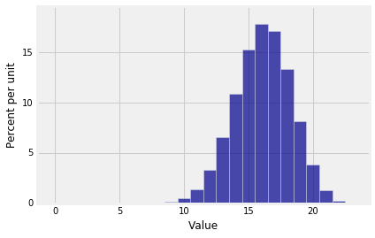
Let's visualize this for a $n = 23$ and $p = 0.7$, two parameters that have no significance other than being our choice to use in this example.
n = 23
p = 0.7
k = range(n+1)
bin_23_7 = stats.binom.pmf(k, n, p)
bin_dist = Table().values(k).probability(bin_23_7)
Plot(bin_dist)
# It is important to define k as an array here,
# so you can do array operations
# to find all the ratios at once.
k = np.arange(1, n+1, 1)
((n - k + 1)/k)*(p/(1-p))
What Python is helpfully telling us is that the invisible bar at 1 is 53.666... times larger than the even more invisible bar at 0. The ratios decrease after that but they are still bigger than 1 through $k = 16$. The histogram rises till it reaches its peak at $k = 16$. You can see that $R(16) = 1.1666 > 1$. Then the ratios drop below one, so the histogram starts going down.
We can solve an inequality to show that the largest $k$ for which $R(k) \ge 1$ is the integer part of $(n+1)p$. In our example, this is $k = 16$ because
(n+1)*p
Mode of the Binomial
A mode of a discrete distribution is a possible value that has the highest probability. There may be more than one such value, so there may be more than one mode.
For all $k$ such that $R(k) \ge 1$, we will say that the binomial histogram is either rising or flat at $k$. The largest $k$ for which $R(k) \ge 1$ has to be a mode; for all larger $k$, the histogram will be falling.
Let $q = 1-p$. Every value $k$ for which $R(k) \ge 1$ must satisfy $$ \big{(} \frac{n+1}{k} - 1 \big{)} \frac{p}{q} ~ \ge ~ 1 $$ That is, $$ \frac{n+1}{k} ~ \ge ~ \frac{q}{p} + 1 ~ = ~ \frac{1}{p} $$ which is equivalent to $$ k ~ \le ~ (n+1)p $$
Therefore the largest $k$ for which $R(k) \le 1$ is the integer part of $(n+1)p$. That's a mode of the binomial.
Because the odds ratios are non-decreasing in $k$, the only way in which there can be more than one mode is if there is a $k$ such that $R(k) = 1$. In that case, $P(k) = P(k-1)$ and therefore both $k$ and $k-1$ will be modes. To summarize:
The Mode
The mode of the binomial $(n, p)$ distribution is the integer part of $(n+1)p$. If $(n+1)p$ is an integer, then $(n+1)p - 1$ is also a mode.
But in fact, $np$ is a more natural quantity to calculate. For example, if you are counting the number of heads in 100 tosses of a coin, then the distribution is binomial $(100, 1/2)$ and you naturally expect $np = 50$ heads. You don't want to be worrying about $101 \times (1/2)$.
You don't have to worry when $n$ is large, because then $np$ and $(n+1)p$ are pretty close. In a later section we will examine a situation in which you can use $np$ to get an approximation to the shape of the binomial distribution when $n$ is large.